Network Analysis

Nathan Sylte
4/21/2017

Sand Mine Road Cost Analysis

Background and Objectives:

The primary objective of this assignment is to become familiar with network analysis. This involved performing a transportation cost analysis on the hauling of frac sand on roadways as part of the ongoing sand mine suitability project. The intention was to route sand from the sand mines themselves to the nearest railroad terminal. It should be pointed out that some of the specifics as far as cost are just hypothetical, and were used for the purpose of learning network analysis. Therefore, the number of trips the haul trucks took was estimated as well as the overall cost.

An additional portion of the assignment that took take place before the network analysis involved generating a python script. This was done to prepare some of the data that was used for the network analysis portion of the project. The utilization of python allowed the initial data to be processed in a fast and efficient manner.

Methods:

The steps for the project can be laid out in the following order.

• Generate a python script that will select active mines, mines that do not have a rail loading station on site, and mines that are not located within 1.5 km of a rail line.
• Use model builder to calculate the closest facility route. This will be done by using the data generated from the python script and a ESRI Street Map USA dataset.  
• Calculate the transportation cost of sand truck travel on the roads by county.
• Generate a map showing the sand transportation routes and costs by county.

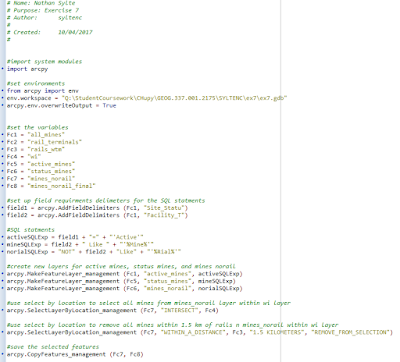
To begin the project a python script was created using PyScripter (Python Script ). This model selected active mines, mines that did not have a rail loading station on-site, and mines that were located further than 1.5 km away from a rail line (Figure 1).

Figure 1. Python script for network analysis assignment.

Next, with the use of model builder the closest route from the sand mine to the rail facility was calculated. Also, the transportation costs to haul the sand were calculated per county. The model is shown in Figure 2.

Figure 2. Data flow model calculating the closest route from the sand mine to the fail facility. Also, shows the calculated cost per county.

First, the closest facility layer was added and the ESRI Streets layer was used as the input. Next, the add location tool was used to specify the mines feature class as the incidents. The same tool was used again to make the rail terminal feature class the facilities. After setting the incidences and facilities, the solve tool was used to create the closest facility routes. The select data tool was then used to select the closest facility routes, and the copy features tool allowed the facility routes to be made into a new feature class. After the routes feature class was created, the routes feature class was projected into the correct coordinate system so it could then be intersected with the county boundaries feature class.

A new field was then added to the county boundaries / routes intersect. This field was named distance. The calculate field tool was then used to determine the total distance traveled on each of the routes on a per county basis. The following equation was used [Shape_length] * 0.00621371. This equation also converted meters into miles. Following this another filed was added. This field was called the annual cost field. Again, calculate field was used to calculate the annual cost per county. The following equation was used ( [distance_miles] *100 *.022). The number 100 represents the total amount of trips going to and from the each mine while the cost per mile is estimated at 2.2 cents per mile. After the annual cost was calculated summary statistics was used to determine the total annual cost per county. The COUNTY_NAM  field was selected as the case field and the statistics type that was used was SUM.

Result and Discussion:

Figure 3. Road cost analysis per county. Counties with the greatest cost are shown in dark orange/brown while counties with no sand transportation costs are shown in tan. Annual cost is in dollars and is only hypothetical.

Chippewa County represented the county with the highest annual sand transportation cost (Figure 3). There are many sand mines in Chippewa County and there is also a rail terminal. This contributes to high road usage by sand trucks. Trempealeau County also had a high annual transportation cost. There are many sand mines located in Trempealeau County, however, when compared to the mines in Chippewa County they are located closer to rail terminals. Overall, sand mine activity is primarily located in the Northwest/Central part of the state. Refer to the first blog post for information as to why this is Sand Mining in Western Wisconsin . Therefore, many counties do not have any costs related to sand mining.

Total cost per county is also shown below (Figure 4, Figure 5).

Figure 4. Total cost per county shown in excel.

Figure 5. Bar graph generated in excel showing total transportation cost per county.

Conclusion:

Overall, network analysis proved to be a very applicable and useful tool. This tool could also be applied to a number of different projects other than the sand mine road cost analysis. Furthermore, model builder was very useful on this project. It allowed the user to keep track of every tool that was used, and kept the data analysis portion of the project organized. This was important because on several occasions the model had to be changed. A future project could use network analysis to determine the quickest driving routes around sand mine rail terminals since the trains can be quite long.