Raster Modeling: Sand Mine Suitability and Risk

Nathan Sylte
5/16/17

Raster Modeling 

Goals and Objectives:

As the final part of the ongoing sand mine suitability project the overall objective was to determine suitable areas for sand mining with the use of raster analysis. Due to the controversy and potential hazards surrounding sand mining (Sand Mining ), a risk assessment was also performed. Therefore, if a mine location was suitable the potential risk the mine posed on the surroundings was assessed. 

The criteria and objectives for sand mine suitability was determined and is listed as below. 

• Generate a spatial data layer to meet geologic criteria
• Generate a spatial data layer to meet land use land cover criteria
• Generate a spatial data layer to meet distance to railroads criteria
• Generate a spatial data layer to meet the slope criteria
• Generate a spatial data layer to meet the water-table depth criteria
• Combine the five criteria into a suitability index model 
• Exclude the non-suitable land cover types  

The correct geology is important because not all sand is of the quality required for mining. The Jordan and Wonewoc formations were selected as quality areas. Another important factor for determining suitability was the current land use. Urban and developed areas would represent areas that were highly unsuitable for sand mining. Rail proximity was also important. The closer the mine could be located to a rail sight the more cost effective the mine could be. Mines would also have to be located in areas that possessed a moderate slope. Areas with a high slope could potentially hinder mining operations. Finally, sand mines need to use great quantities of water for cleaning the sand. Therefore, mine locations were chosen in areas that have a very high water table. 

The criteria and objectives for sand mine risk was determined and is listed below.

Generate a spatial data layer to measure impact to streams

Generate a spatial data layer to measure impact to prime farmland 10

Generate a spatial data layer to measure impact to residential or populated areas

Generate a spatial data layer to measure impact to schools

Generate a spatial data layer to measure impact on wildlife areas 

Combine the factors into a risk model 

As previously stated, sand mines pose a potential risk to the surrounding area. Streams are an important natural resource and can potentially be polluted and impacted by sand mining. Proximity to streams was assessed by taking large to moderate streams and creating a risk index surrounding those streams. The further away from a stream the less risky. Farmland is another key natural resource that is important to Trempealeau. Areas of prime farmland were identified by determining areas that were highly erodible or not. Areas that were not highly erodible represented areas of prime farmland. These areas would receive a high risk factor. Due to noise and potential pollution, mines that could potentially be located next to urban areas would possess a high amount of risk. Therefore, urban areas were assigned as areas of high risk. Trempealeau County possesses several schools located in rural areas. This is why schools were included in the risk assessment. Mines that could potentially be near schools would present a high risk to that particular school. The final risk factor that was included in the assessment was the proximity to wilderness areas. Wilderness areas are an important and dwindling natural resource that are frequently shared by the public. Therefore, due to the potential impact that sand mining could have an wilderness areas, these areas were selected as areas of high risk. Finally, the suitability and risk models were to be combined to determine the best possible areas for sand mining. 

Methods:

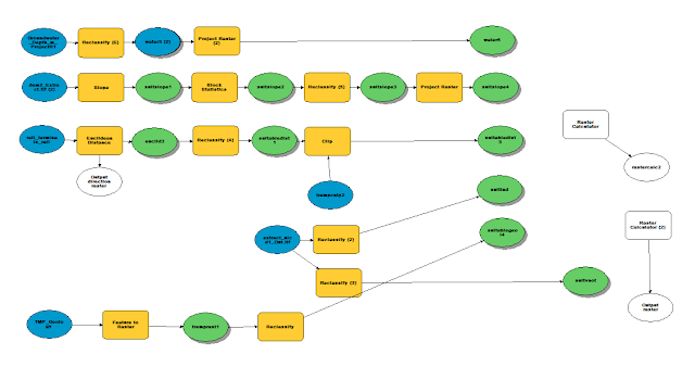
Model builder was used to generate the results to the correct specifications. Figure 1 below shows the model that was used to determine sand mine suitable areas. 

Figure 1.

First, the ideal locations that possessed the correct ground water depth were determined. This was done by converting the geology features to a raster format. The reclassify tool was then used to classify areas with ground water close to the surface, moderate groundwater depth, and deep ground water depth. 

Next, the Trempealeau County DEM was used to calculate areas with adequate slope. The slope and block statistics tools were used to determine the correct slope values. The reclassify tool was used to separate the slope values into highly, moderate, and low suitability areas. 

After the slope was calculated, proximity to rail lines was determined. The rail terminals class was imputed into the euclidean distance tool. The distances were then reclassified into areas that were close, moderately close, and far away from rail terminals. 

Suitable land was then calculated. This was done in two steps. First, areas that were completely unsuitable for sand mining such as urban areas were determined and would later be excluded. The other areas were then separated into three classes where the most highly suitable areas were baron and undeveloped land. 

Finally, adequate geology was determined. Areas of the Jordan and Wonewoc formations were selected as highly suitable and the other areas were marked as unsuitable. The raster calculator tool was then used to add the five previous rasters together. This would make a map that showed areas that were suitable for sand mining. 

Model builder was further used to calculate risk and merge the suitability and risk models (Figure 2).

Figure 2.

Proximity to streams was calculated by using the euclidean distance tool, then areas around the streams were reclassified into areas either close to, moderately, or far away from streams. 

Prime farmland locations were determined by first changing the feature class into a raster by using the polygons to raster tool. In this instance areas that were high erodible were selected as areas poorest for farming. The reclassify tool was then used to separate areas into prime, moderate, and poor farming locations. 

Next, urban risk was assessed by using the euclidean distance tool to calculate distance. Areas within 640 meters of urban areas were selected as high risk areas. This was included in the reclassify tool. As for assessing the risks on schools, the schools had to be converted into a raster format by using the polygons to raster tool. The same procedure was then used to calculate the risk on schools as the was the risk on urban areas where areas within 640 meters of schools were selected as high risk areas. 

After risk to urban areas and schools were assessed, the potential sand mine risk to wildlife areas was calculated. The feature to raster tool was used to convert the data into the proper format. Then euclidean distance was implemented to determine land proximity to wilderness areas. When the areas were reclassified, locations within 1000 meters of a wilderness areas where selected as high risk.

Finally, raster calculator was used to add the five risk raster together to yield which areas were at the highest risk to sand mining. Both the risk and suitability models were reclassified and added together using the raster calculator. This final result showed which areas were best for sand mining. 

Results and Discussion:

 Below in Figure 3 are the five different suitability factors. As displayed below Trempealeau County contains a large amount of the Jordan and Wonewoc formations. A large portion of the county also possessed a very high water table where the proper sandstone are located. Overall, the county contains large areas of either suitable or highly suitable land. However, areas in the northern and eastern sections of the county are located far away from any rail terminals. This could potentially cause issues with removing the sand from the mine location. 

Figure 3. Suitability models for sand mining in Trempealeau County. 

Below in Figure 4 are the five different risk factors. Trempealeau County has many streams, this is evident by looking at the proximity to streams results. Large portions of the county are located near streams. On the other hand, many areas of the county are highly erodible. It should also be noted that there are many, although not large, portions of the county that are located near schools and wilderness areas. Overall, the largest risk sand mining imposes is on stream health. 

Figure 4. Risk factors for sand mining in Trempealeau County. 

Below are the suitability and risk models (Figure 5). 

Figure 5. Suitability and risk models. 

The final result was the combination of the suitability and risk models (Figure 6). Displayed in red are the best areas for sand mining. As seen below Trempealeau County contains many areas that possess the correct conditions for sand mining. Although the county contains many of the correct areas for mining, these areas of often located near some of the worst areas for mining. Overall, the best locations to put sand mines in Trempealeau County are in the west central portion of the county. The worst areas to put sand mines in Trempealeau County are located in the southern portion of the county. 

Figure 6. Final sand mine model showing the best mine locations. 

Conclusion:

Although there is much controversy surrounding sand mining in Wisconsin, it has been demonstrated that there are some low risk areas to mine. The final decision to sand mine will have to be made by the local populations, and proper assessment and planning will be critical. Therefore, if a mine were to open operations in an area it will pose the lowest amount of risk and controversy. 

Network Analysis

Nathan Sylte
4/21/2017

Sand Mine Road Cost Analysis

Background and Objectives:

The primary objective of this assignment is to become familiar with network analysis. This involved performing a transportation cost analysis on the hauling of frac sand on roadways as part of the ongoing sand mine suitability project. The intention was to route sand from the sand mines themselves to the nearest railroad terminal. It should be pointed out that some of the specifics as far as cost are just hypothetical, and were used for the purpose of learning network analysis. Therefore, the number of trips the haul trucks took was estimated as well as the overall cost.

An additional portion of the assignment that took take place before the network analysis involved generating a python script. This was done to prepare some of the data that was used for the network analysis portion of the project. The utilization of python allowed the initial data to be processed in a fast and efficient manner.

Methods:

The steps for the project can be laid out in the following order.

• Generate a python script that will select active mines, mines that do not have a rail loading station on site, and mines that are not located within 1.5 km of a rail line.
• Use model builder to calculate the closest facility route. This will be done by using the data generated from the python script and a ESRI Street Map USA dataset.  
• Calculate the transportation cost of sand truck travel on the roads by county.
• Generate a map showing the sand transportation routes and costs by county.

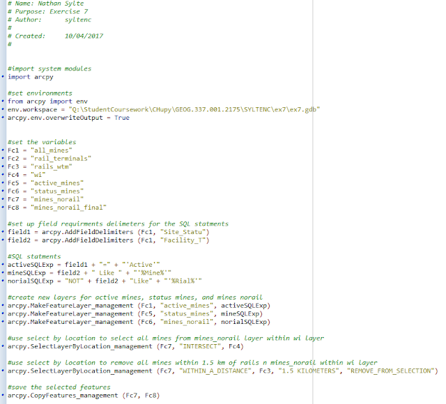
To begin the project a python script was created using PyScripter (Python Script ). This model selected active mines, mines that did not have a rail loading station on-site, and mines that were located further than 1.5 km away from a rail line (Figure 1).

Figure 1. Python script for network analysis assignment.

Next, with the use of model builder the closest route from the sand mine to the rail facility was calculated. Also, the transportation costs to haul the sand were calculated per county. The model is shown in Figure 2.

Figure 2. Data flow model calculating the closest route from the sand mine to the fail facility. Also, shows the calculated cost per county.

First, the closest facility layer was added and the ESRI Streets layer was used as the input. Next, the add location tool was used to specify the mines feature class as the incidents. The same tool was used again to make the rail terminal feature class the facilities. After setting the incidences and facilities, the solve tool was used to create the closest facility routes. The select data tool was then used to select the closest facility routes, and the copy features tool allowed the facility routes to be made into a new feature class. After the routes feature class was created, the routes feature class was projected into the correct coordinate system so it could then be intersected with the county boundaries feature class.

A new field was then added to the county boundaries / routes intersect. This field was named distance. The calculate field tool was then used to determine the total distance traveled on each of the routes on a per county basis. The following equation was used [Shape_length] * 0.00621371. This equation also converted meters into miles. Following this another filed was added. This field was called the annual cost field. Again, calculate field was used to calculate the annual cost per county. The following equation was used ( [distance_miles] *100 *.022). The number 100 represents the total amount of trips going to and from the each mine while the cost per mile is estimated at 2.2 cents per mile. After the annual cost was calculated summary statistics was used to determine the total annual cost per county. The COUNTY_NAM  field was selected as the case field and the statistics type that was used was SUM.

Result and Discussion:

Figure 3. Road cost analysis per county. Counties with the greatest cost are shown in dark orange/brown while counties with no sand transportation costs are shown in tan. Annual cost is in dollars and is only hypothetical.

Chippewa County represented the county with the highest annual sand transportation cost (Figure 3). There are many sand mines in Chippewa County and there is also a rail terminal. This contributes to high road usage by sand trucks. Trempealeau County also had a high annual transportation cost. There are many sand mines located in Trempealeau County, however, when compared to the mines in Chippewa County they are located closer to rail terminals. Overall, sand mine activity is primarily located in the Northwest/Central part of the state. Refer to the first blog post for information as to why this is Sand Mining in Western Wisconsin . Therefore, many counties do not have any costs related to sand mining.

Total cost per county is also shown below (Figure 4, Figure 5).

Figure 4. Total cost per county shown in excel.

Figure 5. Bar graph generated in excel showing total transportation cost per county.

Conclusion:

Overall, network analysis proved to be a very applicable and useful tool. This tool could also be applied to a number of different projects other than the sand mine road cost analysis. Furthermore, model builder was very useful on this project. It allowed the user to keep track of every tool that was used, and kept the data analysis portion of the project organized. This was important because on several occasions the model had to be changed. A future project could use network analysis to determine the quickest driving routes around sand mine rail terminals since the trains can be quite long.

Geocoding and Error Assessment

Nathan Sylte
4/7/17

Geocoding 

Background and Objectives:  

As a section of the multi-part sand mine suitability/risk model project, this part of the project will continue to focus on sand mining in Wisconsin. Trempealeau County will continue to be a focal area of the project. However, in this section of the project the study area was expanded to other areas in Western Wisconsin. The primary objective of this section is to geocode sand mine addresses with the use of a normalized data table. Sand mine location data was provided by the Wisconsin DNR, however, the data had to be normalized before they could be used for geocoding. 

The overall objectives for the lab are as follows:

•  Normalize the mines MS Excel table.
•  Connect to the geocoding service from ESRI and geocode the assigned mines. 
•  Connect to the departmnt ArcGIS server and add the Public Land Survey System (PLSS) feature class. 
•  Manually locate the assigned sand mine locations using either their address or PLSS location. 
•  Compare results with the actual sand mine locations as well as with other colleagues results. 

Methods:

To begin the sand mine location data table that was provided had to be normalized. The original data table contained several errors that had to be corrected before geocoding could take place (Figure 1). Spaces in the titles had to be removed and certain information such as addresses as well as PLSS locations had to be separated so they were alone (Figure 2). 

Figure 1. Original data table (not normalized). 

 Figure 2. Normalized data table with address and PLSS information separated. 

Next, the sand mine locations were geocoded. This was performed by logging into the enterprise ArcGIS Online Account in ArcMap. The normalized data table that was added into ArcMap was used to geocode, and was selected in the geocode addresses module. After the geocoding tool was ran the address inspector was viewed. Each candidate was viewed individually to see if the mine was indeed in the position that the geocoding results said it was in. Mines that were in the wrong location were manually re positioned using the pick address from map function. Some maps did not have an address provided. For these situations the PLSS location was used to determine were the actual mine location was. In other instances the address that was provided was not were the actual sand mine was. The mine location was set were the drive way met the road way for analysis purposes.

After the sand mines were georeferenced the results were compared to the actual locations of the sand mines. The actual locations were provided by the DNR. Results were also compared with other people in the class that were assigned the same mines. To acquire the information about the distance between the geocoded mine locations, the actual mine locations, and class mine locations, two selections were first performed. The selections were done to select for the mines that were assigned so that a direct comparison could take place (Figure 3). Mines were selected by using the Unique_ID field.

Figure 3. Selection tool.

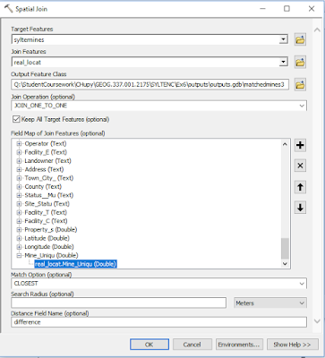
After the correct mines were selected two spatial joins were performed to acquire the distance information (Figure 4). One join was performed between the geocoded mine locations and the actual mine locations. The other spatial join was performed between the geocoded mine locations and the class mine locations. To allow for the correct distance units to be used, the sand mine location data had to be projected into the NAD_1983_Wisconsin_TM (meters) coordinate system. 

Figure 4. Example of one of the spatial joins. 

Following the spatial joins the difference in distance between the mine locations was viewed and then transferred to an Excel spreadsheet for analysis. A map of the mine locations was also generated. 

Results/Discussion:

The primary objective of the lab was to accurately geocode the sand mine locations. Below is a table showing distance between the mine locations (Figure 5). The average distance between my mine locations and the actual locations was around 3000 meters. This is much smaller compared to the distance between my mine locations and the locations of the class mines. The indication of this result is that I was more accurate in placing mine locations than the others in the class who shared the same mines. 

Figure 6 displays were I put the sand mine locations compared to the actual locations. A great majority of the locations were correct. However, two locations in Barron County and one location in Jackson County were incorrect. The reason for this is that there was no mine located were the PLSS data said the mine was supposed to be. The DNR website was used to place these three mine locations which turned out not to be the actual locations. A likely possibility is that these mines are no longer active. The locations on the DNR website may have just been active mines owned by the same company. 

A reason for the large distance (3000 meters) between were I placed the mine locations and the actual mine locations has to do with were I placed the address. The address was placed were the driveway met the main road, whereas, the DNR placed the mine location directly on top of the mine itself. This would account for a good portion of the error. 

 Figure 5. Table showing the distances between the locations of my mines and the actual locations, as well as the distances between my mines and locations were the class put the mines. The right side is the distances between my mines locations and the class mines locations. 

Figure 6. Map displaying geocoded mine locations compared to the actual mine locations as provided by the WIDNR. 

Conclusion:

Overall, the lab was very effective in teaching how to geocode. Geocoding is an important skill to posses and should prove useful in the future. In the future, making sure every location is exactly were it should be will be the primary focus. The lab was also very helpful because required the data to be normalized. Normalizing data is often overlooked even though it is extremely important. If ones data is not normalized then it cannot be used in ArcMap.

Gathering Data: Sand Mine Suitability in Trempealeau County

Nathan Sylte
03/14/17

Gathering Data

Introduction:

The objective of this lab was to re-orient with the method of collecting data from internet sources. Also, part of the objective was to import the data into ArcGIS, join the data, and project data from these different sources into one coordinate system. A geodatabase to store the data was also created.

The scenario involved the first of several steps in an ongoing project. The project is to build a suitability and risk model for sand mining in Wisconsin. As discussed in a previous post about sand mining in Wisconsin, sand mining is very controversial. This makes the suitability and risk model of sand mining in Wisconsin very important.

Overall, the objectives can be laid out in the following manner.

1. Download data from different websites.

2. Import the data and join certain tables.

3. Create a python script to project, clip, and load all of the data into the geodatabase that was created.

Methods:

Data for the project first had to be retrieved and downloaded from online sources. The following sources used are numbered below. After the data were downloaded the data were unzipped and then extracted. The data were then loaded into the proper geodatabase.

1. (U.S. Department of Transportation). The first data retrieved was United States rail lines data. This data was located on the U.S DOT web page. USA DOT Website . After reaching the site the polyline feature class was selected to download the railway data.

2. (USGS National Map Viewer). Next, the 2011 National Land Cover Database was used to download land cover data for Trempealeau County, Wisconsin LandCover Data . Elevation data for Trempealeau Country was also retrieved from this site.

3. (USDA NASS Geospatial Data Gateway). The land crop cover data was found on the US Department of Agriculture website USDA CropCover. The Trempealeau County soil data was then navigated to.

4. (USDA NRCS Web Soil Survey). After going to the webpage USDA web soil survey, Trempealeau County was selected as the AOI (area of interest). Then the soils data was simply downloaded.

5. (Trempealeau County Land Records). Trempealeau County data was found on the Trempealeau County website Tremp County Data. The entire Trempealeau County geodatabase was downloaded.

After the data were downloaded py.scripter/python code was used to create three separate output rasters. The output rasters are results from the DEM model, Crop-cover data, and the Land-cover data. Python Code can by found here Python Script.

Results:

A map was created from the three output rasters which shows crop cover, general landcover, and elevation (Figure 1). Trempealeau County is located in a very hilly region. There are many hill or "bluffs" in Trempealeau County which can be clearly seen on the DEM. The landscape was also dominated by deciduous forest mixed with agricultural fields. Accounting for the southern border of the county is the Mississippi River which provides a large amount of wetland habitat.

Figure 1.

Data Accuracy:

The data accuracy was assessed based off of the metadata provided. Certain metadata was difficult to locate such as Planimetric Coordinate Accuracy. Metadata are shown in the table below (Figure 2).

Figure 2. Metadata displayed. Certain metadata proved difficult to locate and is marked as NA.

Conclusion:

There are great amounts of data that are available online. Understanding how to properly download online data is an important skill that should be utilized when completing a project. Furthermore, many online datasets and datasets in general are extremely large. Working with the data can become time consuming. Therefore, utilizing python scripter to perform various processes on the data can save time. Utilizing python becomes more important the larger the dataset gets. Finally, metadata should always be collected from online datasets. This gives indication into the data integrity. If the dataset does not have any metadata associated with it then there is cause for concern.



Python Scripts (Ongoing script)

Nathan Sylte
3/17/14

Python Script 1 for Exercise 5: Sand Mine Suitability in Treampealeau County

Introduction: Utilizing Python Scripts 

The objective for the following exercises is to gain experience utilizing python scripts to perform various tasks in GIS. Becoming acquainted with PyScripter and the coding language required to use PyScripter will be an important skill to have in the geospatial field. Utilizing python is a necessity to save time and increase efficiency which is extremely important when working with large quantities of data.  

Results: Python Script 

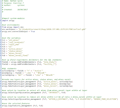
Below is the resulting python script from the Gathering Data: Sand Mine Suitability in Trempealeau County lab shown in notepad (Figure 1). 

Figure 1. Python Script 

The beginning of the script sets up the system modules and sets the environmental settings. The location of the three rasters that I was going to project and extract was set as the environment. Next, the rasters were looped into a different (new) folder using the listOfRasters function. The ProjectRaster_managment function was used to project the rasters in the desired coordinate system. Following this, the rasters were extracted to the boundary of the Trempealeau County. Last, the RasterToGeodatabase function was utilized to place the output rasters in the TMP (Trempealeau County) geodatabase. The outputs can be viewed at Sand Mine Suitability. 

Python Script 2 for Exercise 7: Network Analysis 

Below is the resulting python script from the network analysis portion of the ongoing sand mine suitability project (Figure 2). 

Figure 2. Python script for Exercise 7: Network Analysis. 

The script begins by setting up the different variables that will be used later on, and primarily consists the feature classes that will be created. Next, an SQL statement was created to query out the features that were to be used. In this case the query selected active mines, separated out facilities with the word mine in the title, and separated out facilities that did not have the word rail in the title. 

After the query statements were generated, three separate layers were created from the query selections. The mines that were within the State of Wisconsin were then selected by using the "intersect" tool. Mines that were not in the State of Wisconsin were then removed. The last part of the script copied the selection so that a new feature class could be generated. In this case the feature class was called mines_norail_final (Fc8). 

Python Script for Exercise 8: Raster Modeling 

Sand Mining in Western Wisconsin

Nathan Sylte

GIS 2

Sand Mining in Western Wisconsin 

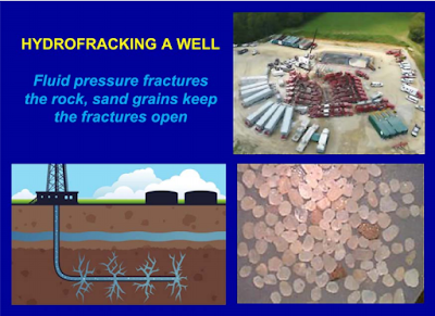
    The mining of "frac" sand in Wisconsin for use in the extraction industry has become an extremely controversial issue throughout the state. Sand mined in Wisconsin is typically used for hydraulic fracturing (fracking) (Figure 2.). Fracking is a technique that is used to extract hydrocarbons such as oil or natural gas that could not otherwise be reached through conventional drilling/extraction methods (Wisconsin DNR).This method for extracting hydrocarbons has been around for 60 years. However, recent advancements in drilling technology have made extracting hydrocarbons with the use of fracking economical in regions where it was previously too costly to extract hydrocarbons. Overall, this post is intended to provide an overview of sand mining in Wisconsin. Several topics will be discussed including the issues and risks associated with sand mining in Wisconsin. An overview of how GIS can be used to investigate sand mining will also be discussed.

    So what is sand mining in western Wisconsin, and why is frac sand mined here? The sand that is used in fracking must meet very specific qualifications. Frac sand must be extremely round and uniform in size (Sand Mining Facts ). The sand must also be pure quartz which makes the sand very hard. The specific strength and size specifications are what allow this type of sand to be used in hydraulic fracturing. Due to these specific specifications frac sand cant be found just anywhere. It just so happens that the correct sand can be found in certain sandstone formations throughout northwest and central Wisconsin. The specific sandstone formations where frac sand can be found includes several Cambrian formations (Wisconsin DNR). These Cambrian formations primarily include the Jordan, Wonewoc, and Mt. Simon Formations (Figure 1). The absolute best sand that can be used in the fracking industry is found in the Jordan formation. The Jordan formation is narrowly found in the southern part of Pierce County and western section of the Chippewa Valley.

    Part of the controversy surrounding frac sand mining includes the methods used to actually mine the sand itself. The procedure involved to mine the sand includes several steps (Wisconsin DNR). First, overburden must be removed to expose the sand. Overburden can describe vegetation and topsoil that are variable in thickness. This step is generally performed by heavy machinery such as scrapers, bulldozers, and excavators. After the sand has been exposed it must then be excavated. Excavation is generally done by large front end loaders and excavators. However, a blasting step is sometimes required to allow the sand to be removed. Blasting involves the use of explosives to loosen the sand for excavation. Blasting has the potential to create dust emissions so steps are taken to reduce those emissions. One of the steps taken to reduce dust emissions involves the use of stemming material, which is used to back fill explosive bore holes.  The last steps involved in the sand mining process involve the crushing and shipping of the sand. Many times the sand must be crushed at the mine site. Crushing is done to further sort the sand into the desired size. After the target sand has been separated the sand is then shipped to a sand processing plant to be processed into frac sand. It is important to include that after the mine is cleared of the desired sand, a reclamation process must occur to restore the area as best as possible. The reclamation process is typically an on going process that is designed to restore topsoil and integrity to the area so that the location can return to as much of a pre-mine state as possible.

    Although steps are taken to mitigate the impact of sand mining. Environmental issues will often arise and can include the following (Wisconsin DNR). The first issue being that of air quality and pollution. Dust and chemicals involved in the handling and processing of the frac sand are often released into the surrounding environment leading to a decrease in air quality. Air quality issues typically arise in the areas around the mine and processing sites themselves.

    Another sand processing activity than can have environmental implications is the washing of the sand at the processing plant (Wisconsin DNR). The process of washing and cleaning the sand involves the use of many thousands of gallons of water. In fact, the washing of the sand can use up to 3,000 gallons of water per minute. It should be added that there are efforts to recycle the water by putting it in holding ponds to be re-used. Despite efforts to re-use as much water as possible, processing plants can have great impacts on the local water tables. A sand processing plant can use up to 2 million gallons of water per day. This has the potential to significantly impact trout streams as well as personal home wells. There have also been many anecdotal references to a sand processing plants ability to severely disrupt local wells and water tables. It should also be added that various chemicals are used during the cleaning process which could have the potential pollute if not properly monitored, contained, and recycled.

    An important impact that frac sand mining can have on the local area has to do with the transportation of the sand. Sand is often transported via dump trucks and semi trucks from the mine site to the processing plant. These heavy vehicles can decrease the longevity of road ways causing millions of dollars in repairs.

    GIS (geographical information systems) software is an important tool involved in the monitoring of sand mining and processing. GIS can be used to monitor environmental impacts and local infrastructure. For example, GIS could be used to monitor regional wells and water table levels around sand processing facilities. The software could also be used to plan trucking routs and monitor the roads the trucks travel on. Databases could be generated in both instances that could be used for analysis purposes. GIS can also be used to map out where the sand mines should go, and provide information on the mines condition. The use of GIS software has the potential to save time and money, as well as increase environmental safety. These factors are ultimately beneficial to the companies and local communities involved in sand mining.

Figure 1. Above is a map of frac sand mines and processing plants throughout the state of Wisconsin A large cluster of sites can be seen in western Chippewa County. This map is provided by the Wisconsin Geological and Natural History Survey. Sand Mining Facts

 

Figure 2. Depicted is the general process of hydraulic fracturing. Also shown is the quartz sand used in the process of fracking. Hydrofracking and Sand Mining

References:

Wisconsin DNR. (2012). Silica Sand Mining in Wisconsin. Retrieved from http://dnr.wi.gov/topic/Mines/documents/SilicaSandMiningFinal.pdf

Wisconsin Geological and Natural History Survey. (2012). Frac sand in Wisconsin. Retrieved from http://wcwrpc.org/frac-sand-factsheet.pdf